In an era of climate change, wildfires have become a focal point of study - particularly for the West Coast. Trends for recent years have not shown much change in the total amount of fires, but they have shown an increase in the amount of land burned by these fires (Wildfire Statistics). The implications can be severe: deforestation, homelessness, and increased carbon emissions, among others.
While it is unlikely that wildfires are preventable, with appropriate action, the damages done can be reduced. To do this, there needs to be proactive action in conjunction with better indicators for wildfire risk. Our project sought to identify these variables and created two predictive models to classify the susceptibility of a state to wildfires. Note that in the scope of this work, susceptibility is directly related to the total number of fires in a specific location. Consequently, the variables were used to create a predictive model that predicts the number of wildfires in a state. Ideally, these results yield meaningful data regarding wildfire severities and frequencies which can be used to schedule and allocate fire prevention resources more effectively.
To collect data, major physical and environmental factors were brainstormed and analyzed using intuition as well as research into existing wildfire papers. Specifically, Chas-Amil M.L’s paper, Natural and Social Factors Influencing Forest Fire Occurrence at a Local Spatial Scale, was a particularly helpful source for determining several factors that were connected to wildfires[1]. Analysis of the paper led to the decision that datasets for the following factors should be collected: temperature, precipitation, humidity, biomass, wind, and human factors.
The first three factors, temperature, precipitation, and humidity were collected for each of the mainland United States on a monthly basis for the timeframe of 2011 to 2020[2]. Alaska and Hawaii were excluded due to their significant spatial disconnect from the rest of the states in addition to having distinct habitats (tundra and tropical island respectively). When considering a mechanism to capture biomass data, forest coverage was chosen[3]. This metric was used on a per state basis and assumed to be consistent across the timespan. The assumption of consistency is reasonable because at the level of state with only a 10 year range there is likely relatively minimal changes to the amount of forestland in each respective state. Wind datasets were found; however, there was a large price to obtain these datasets. Due to budgetary constraints, wind was ultimately excluded from the model. Finally, human factors is a relatively broad term. As such, the population of each state for each year was selected to represent this feature[4]. This parameter is a decent estimate given that statewide data was scarce for other “human factors”.
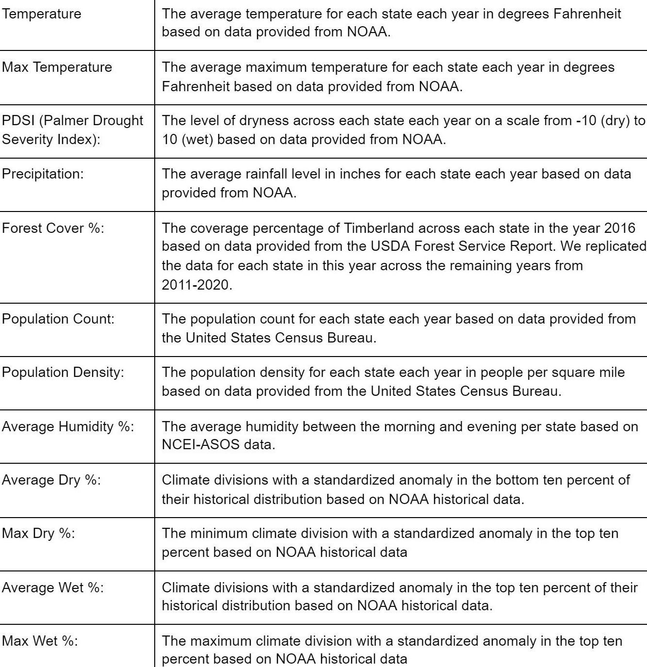
Table 1, shown below, details each variable used and provides a brief description. Note that some variables were derived from a single dataset. For example, max temperature was calculated on a yearly basis from the same data set that average temperature was calculated.
In order to build a predictive model, labels were needed for the purpose of training and prediction. To do this, annual reports for each year from 2011-2020 published by the National Interagency Coordination Center were utilized[5]. These reports gave wildfire counts on a state by state basis for the intercontinental U.S. for each year.
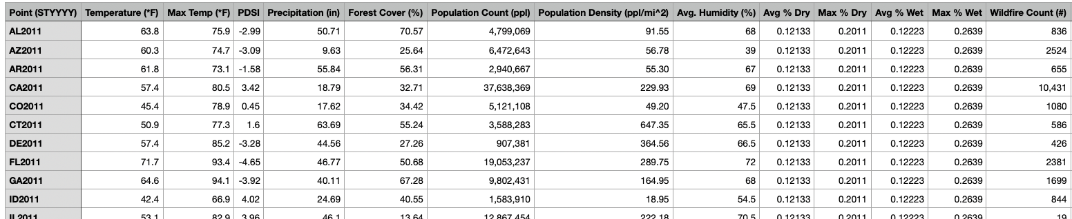
With labels and features for each state each year across a ten year period utilized, processing and cleaning of the data was performed.
These data were all implemented into different sheets and then fully compiled into one sheet to be exported as a CSV file for ease of use with code. The CSV file was imported into clean.py along with the Pandas module. The read_csv() function provided a convenient way to organize all these data into a dataframe. When importing the CSV file, a couple features of the data were incorporated as strings rather than numerical values (int, float, etc.), which were more desirable to model with. Strings would cause problems within the model as the object values would not be feasible for numerical modeling.
Each feature and label was processed in order to eliminate any string objects (and thus turning them into integers or floats) and then incorporated into numpy arrays. To do this, we had a series of conditionals for each feature and the label to check if the column datatype of the dataframe was designated “object”. If so, then the dataframe column values were translated into a list using the toList() function in Pandas then the list was iterated through to eliminate all commas. This list was then translated into a numpy array. If the dataframe column type was not designated “object,” then the dataframe column was incorporated into a numpy array using the to_numpy() function in Pandas. Once the numpy arrays have been created for each list, we implemented a newaxis to each array, specifically to concatenate the features with each other to create a 2-D features matrix using the concatenate() function in numpy. At the end of the data cleaning process, the labels were processed into a (480,1) shape numpy array and the features were processed into a (480,12) numpy array. We had a designated python file for cleaning this data and preparing the matrix for the coding files which implemented our modeling.
With the data cleaned, a correlation matrix (Figure 1) was made by plotting the correlation output between each parameter using the built in correl() function of Google Sheets. The output was a 12 by 12 matrix with each entry corresponding to the correlation between its respective row and column variable. For this reason, the diagonal values were 1, and the matrix is symmetric across the diagonal.
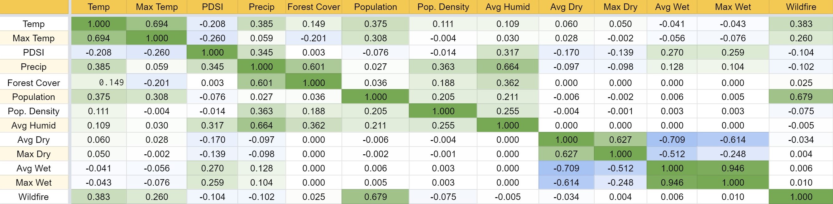
It seemed reasonable that some of the parameters might be connected. For example, temperature might be related to precipitation. It was found that population was the most correlated parameter with the outcome number of wildfires, with a value of .679. Additionally, humidity was related to precipitation with a correlation of .664. Finally, forest cover was found to be closely related to precipitation as well. The output of this matrix signaled that dimensionality reduction could be useful for the model.
Due to the plethora of variables that can go into the creation of forest fires previously stated, dimensionality reduction using principal component analysis was implemented to shrink the number of dimensions in the model, thus simplifying it, while still maintaining effectiveness[1]. The fit and transformation of the dataset was calculated using the PCA class from the skLearn.decompossion module, and reduced the data down to eight principle components. The explained variance for each principal component was then found and summed across the components to ensure 95% of the explained variance was accounted for in the model, enough explained variance to know that this new dataset still accurately represented the original one. This new dataset was then used in different regression models to test the accuracy of the model before and after PCA was applied to the dataset. Afterwards, an unsupervised learning model to cluster the susceptibility levels of states in our study area
The goal when running PCA was to reduce the number of inputs while still accurately representing the dataset. In order to maintain the integrity of the data, 95% of the explained variance needed to be accounted for after the reduction took place.
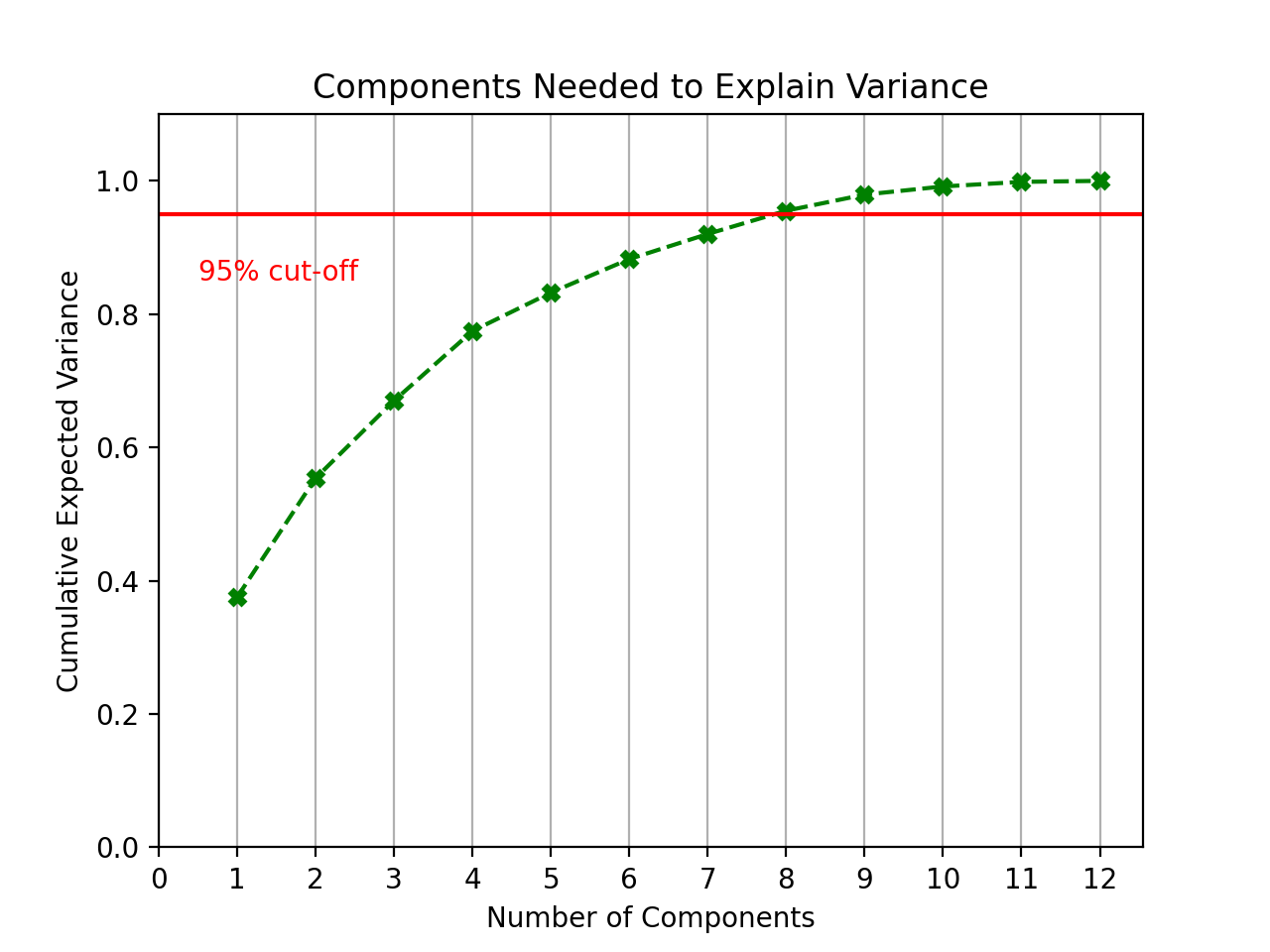
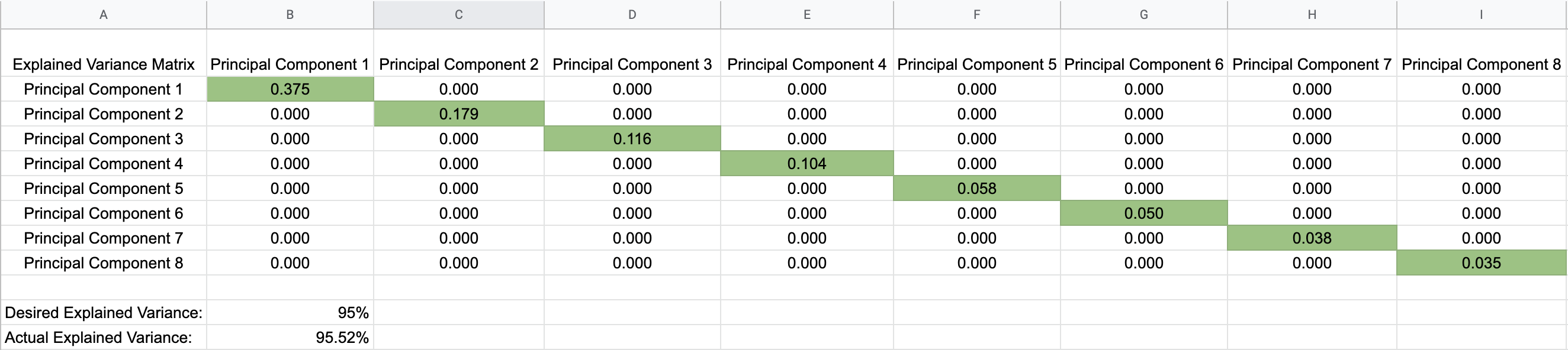
This above graph led to the conclusion that it was possible to safely reduce four dimensions and still maintain the integrity of the data. Below is a matrix showing how each principal component contributed to the total expected variance.
As one of the most common classification techniques utilized in supervised learning models for machine learning, our group chose Naive Bayes as one of the two classification predictive models to implement. In order to get Naive Bayes implemented, all of the data had to be classified into distinct buckets. Because each state in a particular year was classified as either low, medium, or high susceptibility to wildfires, there were three buckets to organize our data into.
For the features, the minimum value and maximum value of each feature was taken and a range for this was calculated. Then organized the data by putting values at < 33% of the range into one bucket, >= 33% and < 66% of the range into the 2nd bucket, and > 66% of the range into the last bucket. Values in each of these buckets were then labeled with 0, 1, or 2 respectively, to represent low, medium or high values for each feature. The same analogy was also implemented for the labels, with 0 representing low susceptibility to wildfires, 1 for medium susceptibility, and 2 for high susceptibility.
The data points were split between 80% training and 20% testing. From here, K-Fold’s method to train and test the data on different parts of the data set was implemented. 5 different iterations were run with 2011 & 2012 used as testing data, 2013 & 2014 used as testing data, 2015 & 2016 used as testing data, 2017 & 2018 used as testing data, 2019 & 2020 used as testing data.
To train the data, the prior probabilities were obtained for each susceptibility level 0, 1, and 2. Afterwards, assignments were made to each testing set data point on the classification of susceptibility by incorporating Bayes’ Rule. The accuracy of our classification by comparing our predicted assignments to the actual ones was recorded. These were done on each fold, and can be found in the Results section. Our Naive Bayes model was implemented on three different instances of the data: one for the full instance of the data, one for an instance after the data was processed through PCA, and one with the positive values denoted in regards to the wildfire counts.
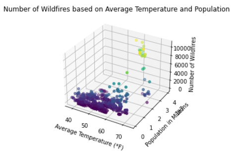
Three sets of data were gathered to be trained and tested by linear regression. The first data set was the originally compiled data with 480 data points consisting of 12 features and one result for the number of wildfires. The second set of data were from the output of the created PCA method which returned 480 data points consisting of eight features and one result for the number of wildfires. The third set of data were taking the same original wildfire data as the original, but with only the columns for average temperature and population size. These two features were deemed the most significant in the correlation matrix. In all three instances, the features were the “x” dataset and the number of wildfires were the ”y” dataset. All datasets were split in two with the first being the first 80% of the data (referring to 2011-2018) which was used for training, and the remaining 20% (referring to 2019-2020) was used for testing. The training data was trained using linear regression on the LinearRegression import from sklearn. Because there can not exist negative wildfires, any negative value predicted from linear regression was replaced with zero.
Logistic regression was handled in a similar fashion to linear regression. After taking in the original set of 480 data points with 12 features and their respective wildfire numbers, a separate dataset was made using the correlation matrix to contain only the 6 variables that most impacted wildfires in a given area (Average Temperature, Max Temperature, PDSI, Precipitation, Population, and Population Density). The two most recent years of data points for both datasets were established as the testing data, with the remaining 80% being allocated for training purposes. Both sets of training data were then used by the logistic regression model, which was imported from sklearn, to fit the model, and ultimately produce predictions on the amount of wildfires for each of the test data points.
The Naive Bayes classification of susceptibility to wildfires proved to be generally accurate, with some folds leading to more accurate classification than others. Classification accuracy results are shown in the table and figure below:
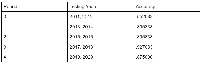
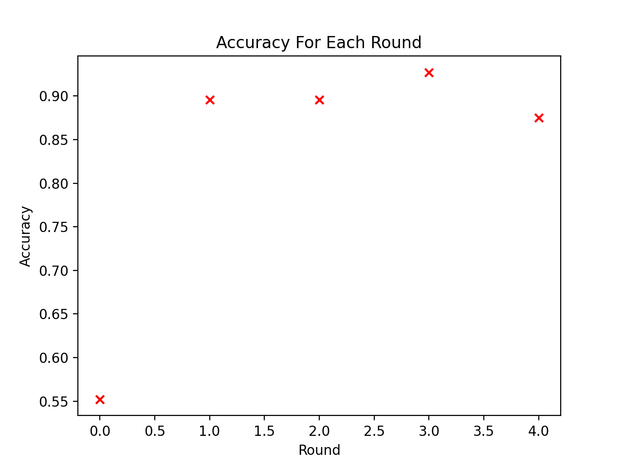
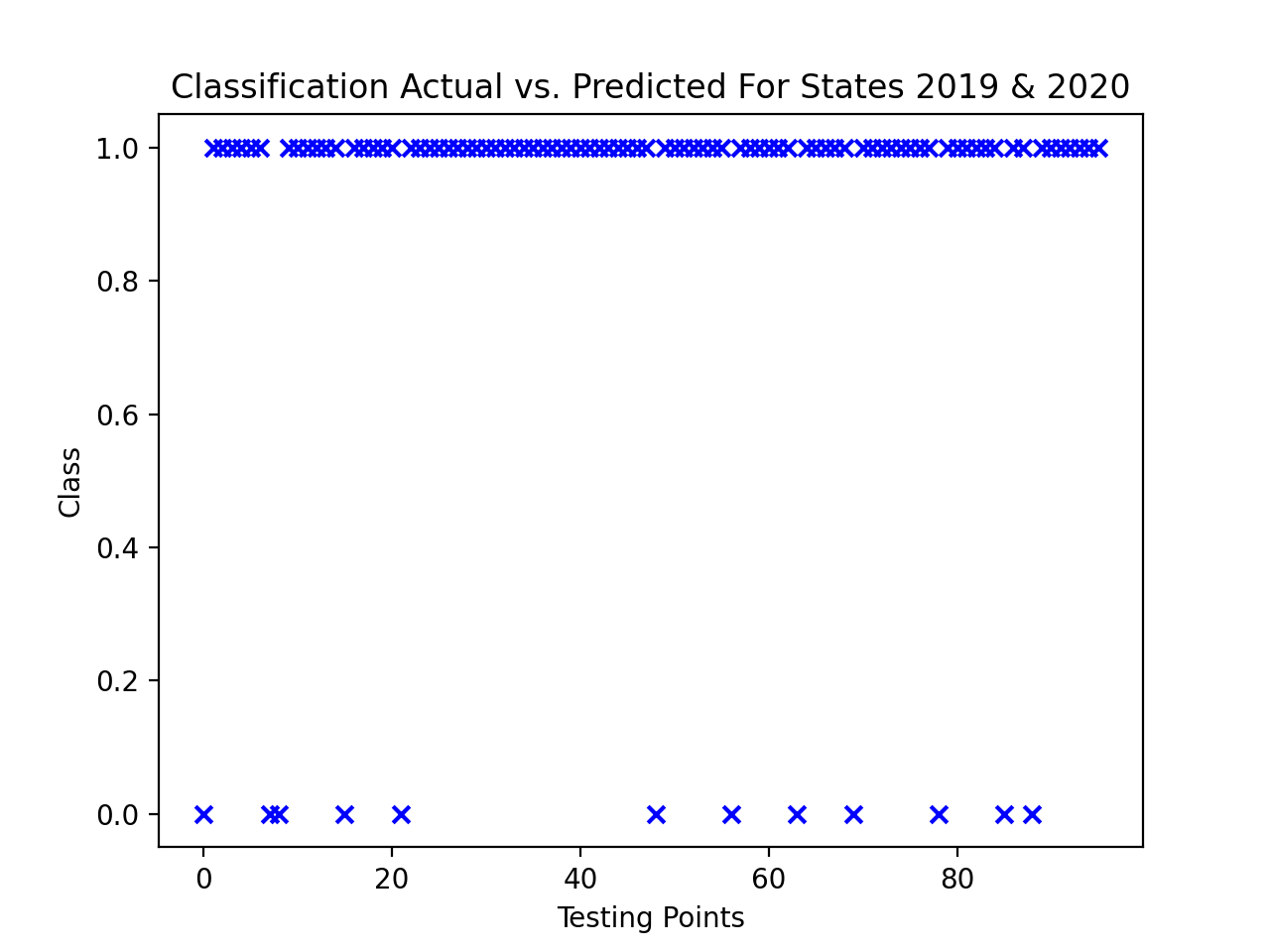
The total accuracy of our classification across all folds was .829167, so overall the Naive Bayes model was quite accurate. But the testing data that was more recent rather than in the past proved to have more accurate results when it came to predicting classification, as using the earliest time periods (2011 & 2012) as testing data showed to lead to more inaccuracies. Below also shows the classification prediction results on the 2019-2020 testing data, where along the class axis, 1 represents a correct classification and 0 represents incorrect classification.
After PCA dimensionality reduction was processed on the features, the prediction results on classification proved to be even more accurate than they were before, which is evidenced in the table and figure below:
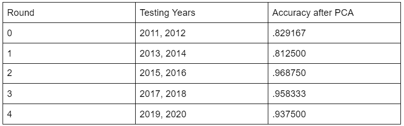
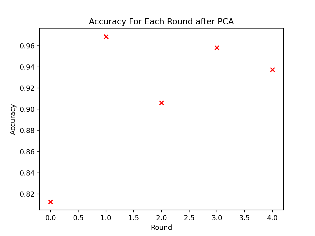
The accuracy results above show that with a reduction in features through PCA we were able to yield more meaningful classification predictions. This is especially the case for the first round, using 2011 & 2012 years for states as testing data. There was a dramatic increase in accuracy here for classification of susceptibility prediction compared to pre-PCA dimensionality reduction. Below also shows the classification results for 2019 & 2020 states used for testing.
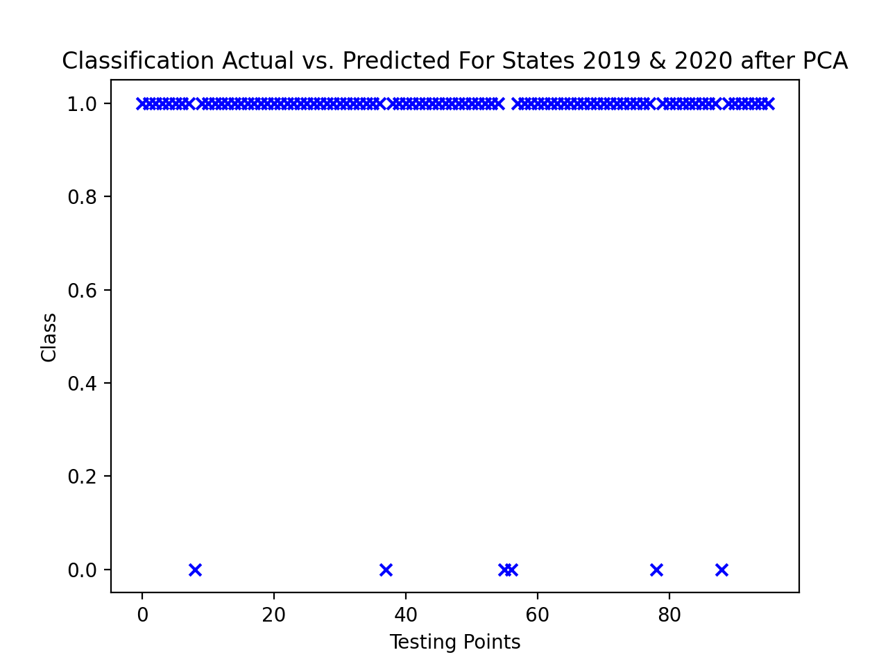
It is evidenced here that while the classification for this testing set after PCA proves to be even better compared to the classification for this testing set before PCA.
The Naive Bayes model was lastly run on the three features that yielded positive values on the correlation matrix in regards to Wildfire. This led to even more accurate results and an improved prediction model compared to both the full instance of data and the data after PCA, as evidenced in the table and figure below denoting the classification accuracy results.
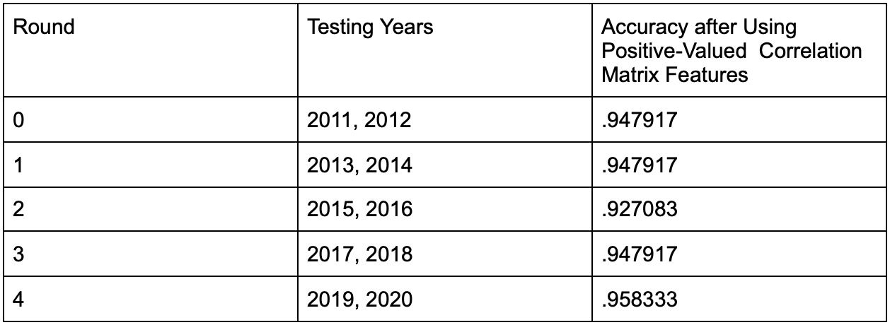
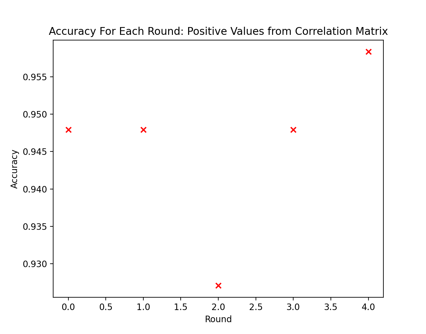
The accuracy results above show that using only the features with positive correlation matrix values in regards to wildfire counts yielded the best results from experimentation. The notable distinction for the positive correlation matrix valued features was evidenced in the 2011-2012 testing years data, where the accuracy was significantly higher than it was for the same testing years in the original instance of data and in PCA. Below also shows the classification results using the years 2019 & 2020 as testing years.
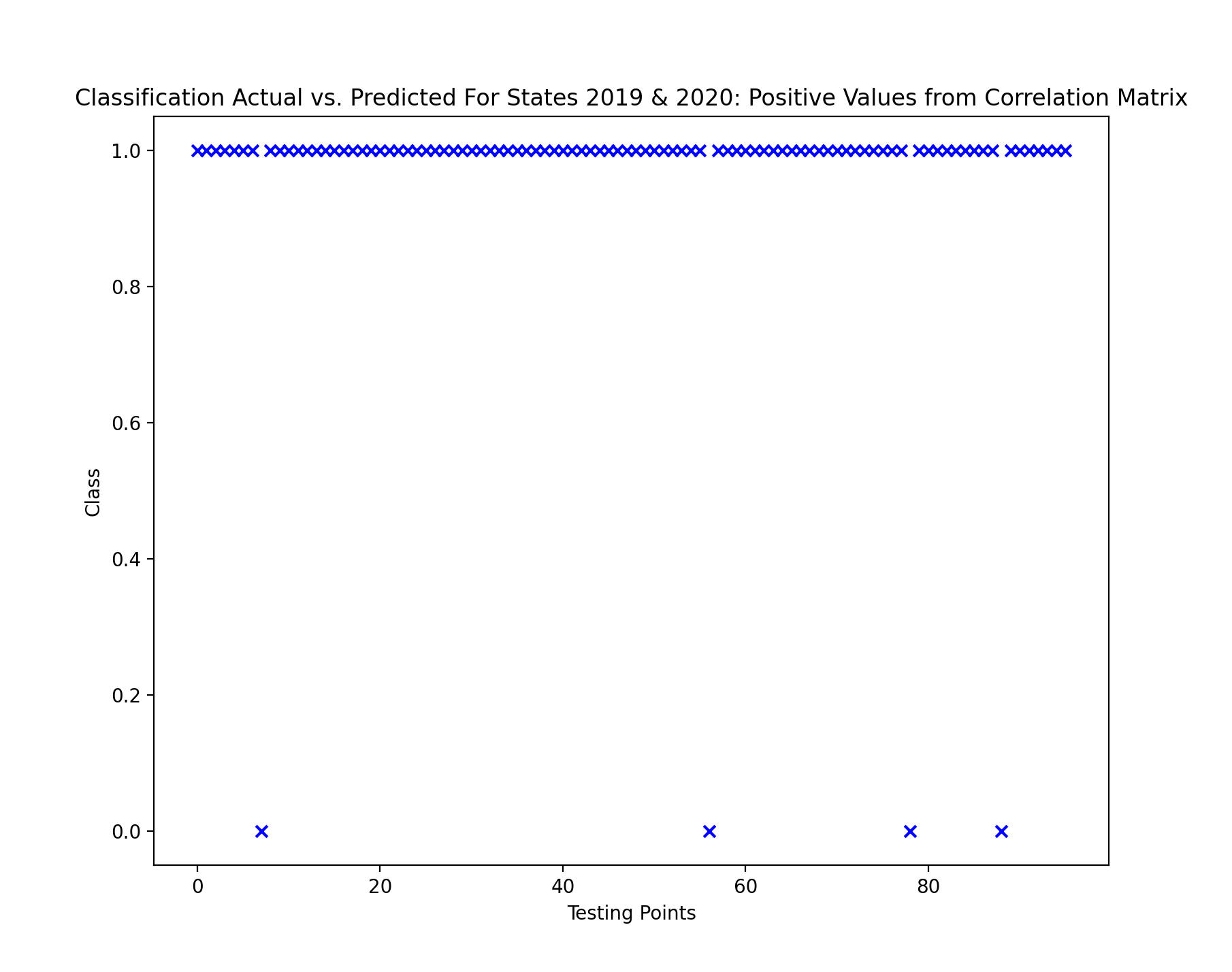
With only four points predicted accurately in the classification, it is evidenced sufficiently that the utilization of the correlation matrix for feature selection proved to be beneficial towards the classification.
With only three features maintained from the positive valued correlation matrix features with respect to wildfire counts, the low amount of features may prove to oversimplify the model, as if additional data values were brought into play, other features would prove beneficial as well. But this gave a good look at the features that were most significant for our model, and classification along these features still yielded the best results. Overall though, it would be best to look at the PCA instance to make use of more features for a much more complex and justified model.
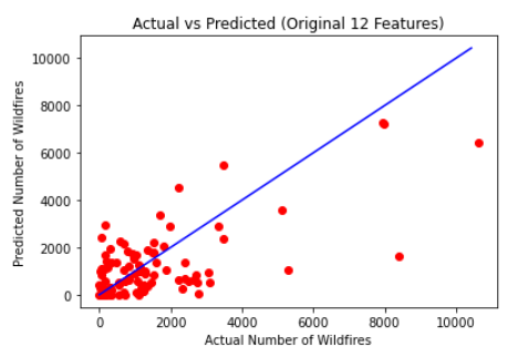
The predicted sets were compared with the test sets to find the root mean square error (RMSE) and R2 values were calculated using mean_squared_error and R2_score functions from sklearn. The RMSE comparing the test set with the predicted set for the original collected data with 12 features was 1412.77 and this data had a R2 value of 0.43393. The test data of this was compared with the predicted data in the graph below. Each red dot’s X coordinate is what that test data’s actual number of wildfires was, and it’s Y coordinate represents how many wildfires were predicted by the linear regression model. The blue line Y=X represents a theoretically completely accurate prediction where the model would predict the same number of wildfires as there actually was for a given state in a given year. This means that the more vertical distance a point is from the line, the more inaccurate the linear regression prediction is. On this first graph, it was found that the predicted exceeded the actual 40 times, under predicted the actual 55 times, and one time got the predicted exactly equal to the actual.
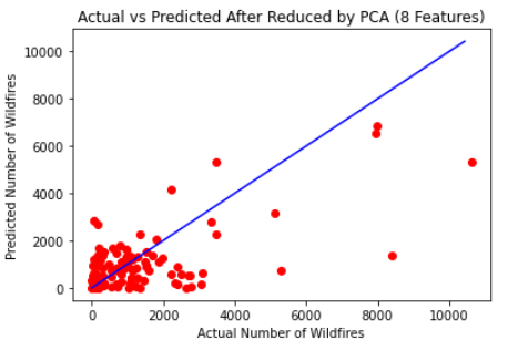
The same process was performed on the data returned by PCA with eight features. This returned a RMSE of 1497.34 and R2value of 0.36413. The same graph from above was recreated below using the post PCA data. The very small difference in RMSE and R2values of the linear regression results between the original 12 feature data and post PCA 8 feature data prove that the feature reduction from PCA does not drastically change and is thus still a valid dataset to form a basis from. On this first graph, it was found that the predicted exceeded the actual 42 times, under predicted the actual 53 times, and one time got the predicted exactly equal to the actual.
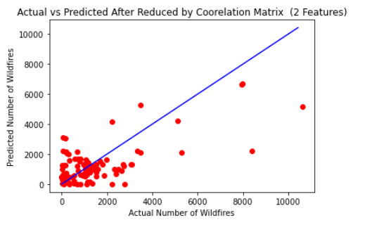
The same process was performed a third time based solely on the data from average temperature and population size. This returned an RMSE of 1415.99 and a R2 value of 0.43134. This very similar result using just two features compared to the original twelve features shows how significant a role these two features played in predicting an outcome in the original which was also shown from the correlation matrix. On this first graph, it was found that the predicted exceeded the actual 43 times, under predicted the actual 53 times, and was never able to get one that had a predicted exactly equal to the actual.
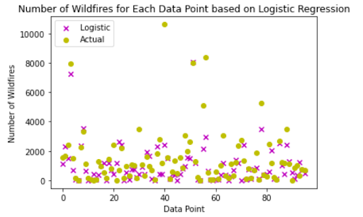
The predicted classifications for wildfires were compared to the actual wildfire statistics for the testing data through both a Root Mean Square Error (RMSE) and R2 using mean_squared_error and R2_score functions from sklearn. After normalizing the data in both the predicted amount of wildfires and actual amount, the RMSE was determined to be 0.14, with an R2 of .48. The results, shown in Figure 13, can be seen comparing the 96 points used in our test data and the logistic regression classifications (shown in magenta) as well as the actual wildfire amounts for each data point (shown in yellow). The logistic regression failed to account for a few outliers, in turn leading to the weaker RMSE and R2.
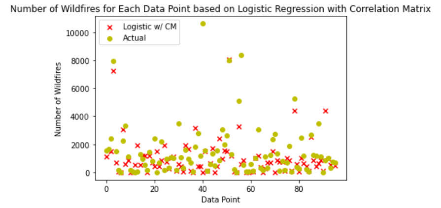
The usage of the dataset containing only the variables that were closely tied to wildfires, as determined by the correlation matrix, produced similar results. After normalizing the data in both the predicted amount of wildfires from this dataset and actual amount, the RMSE was determined to be 0.18, with an R2of 0.37. The results, shown in Figure 14, can be seen comparing the 96 points used in our test data and the logistic regression classifications (shown in red) as well as the actual wildfire amounts for each data point (shown in yellow). The logistic regression failed to account for slightly more outliers, as it had less variables to base its predictions off of, which led to slightly worse RMSE and R2 values.
The data collected was based on the most meaningful factors that were available publicly that could help predict wildfire amounts and susceptibility. While some of the features of data were not as readily available as other features, all of the data was efficiently incorporated and utilized effectively in the model. The models implemented were effective in undergoing more efficient predictions or providing insightful predictions themselves. Final results show generally accurate predictions of both the susceptibility of wildfires through classification and the number of wildfires predicted through linear regression. With the methods implemented, this meaningful predictive analysis will lead to more efficient resource allocation and scheduling routines to help fight and prevent wildfires.
While a bulk of our modeling implementations are complete, there are still a couple things to potentially implement in the future. The supervised learning models on linear/logistic regression as well as Naive Bayes proved meaningful in the goals for classification and prediction. However, looking at additional predictive models such as SVM and Neural Networks could add a potential point of view for wildfire prediction and classification susceptibility levels. In addition, looking at additional feature selection methods, such as forward selection and backward elimination, could give perspective on how different features work together. The data instance itself also could have utilized other potential features that could be important to look into, such as wind speed, vegetation growth, and topography. However, these features weren’t readily available for public usage and required budgetary constraints didn’t work out with obtaining these features either.
Overall though, the predictive models implemented garner a significant basis for predictive analysis. The learning curve behind the development of the models lied not only in the application of unsupervised and supervised machine learning techniques but also the theory behind the implementations. Throughout the course of the project, much time was dedicated not only to the generation of code for the implementations but also understanding the knowledge behind the models developed. Naive Bayes classification techniques on multiple instances of the model demonstrated majority accurate classifications across all instances, demonstrating an eloquent model. Linear Regression across the original 12-feature dataset and the two reduced datasets was overall not a great model at predicting wildfires as seen in the relatively high RMSE values and relatively low R2 values. Despite them not being a great predictive value, they are reasonable given what data is available compared to what other factors also contribute to wildfires that are unable to be obtained. But at the finish, the end goal of building a meaningful prediction model for the benefit of resource allocation and scheduling for better wildfire protection measures was obtained and satisfied.
Machine learning has become an imperative skill to possess in an era of growing technology and societal advancement. One of the best areas this can be applied towards would be the area of natural and manmade disasters that ravage across the United States. Wildfires represent a pinnacle issue in this application area, and the usage of machine learning techniques, both supervised and supervised, towards wildfires serve as a relevant undertaking for investigation. With wildfires becoming a more paramount concern in recent memory, it is imperative that organizations dedicated more sophisticated efforts to the alleviation of wildfires. The predictive models were designed with the intent of contributing to this cause. While there were obstacles present, the potential outcome is meaningful: having a means to predict wildfire impact can save property, the climate, and ultimately, lives.
1. Chas-Amil, Maria Luisa; Touza, Julia M.; Prestemon, Jeffrey P.; McClean, Colin J. 2012. Natural and social factors influencing forest fire occurrence at a local spatial scale. In: Spano, Donatella; Bacciu, Valentina; Salis, Michele; Sirca, Costatino (eds.). Modelling Fire Behavior and Risk. Global Fire Monitoring Center: Freiburg, Germany, 181-186.
2. Climate at a glance. (2021, February). Retrieved March 01, 2021, from https://www.ncdc.noaa.gov/cag/county/mapping.
3. “Home: US Forest Service,” usfs shield. [Online]. Available: http://www.fs.usda.gov/. [Accessed: 05-Apr-2021].
4. U. S. C. Bureau, “Evaluation Estimates,” The United States Census Bureau, 21-Dec-2020. [Online]. Available: https://www.census.gov/programs-surveys/popest/technical-documentation/research/evaluation-estimates.html. [Accessed: 04-Apr-2021].
5. “Coordination and cooperation in wildland fire management.,” Welcome to the Nation's Logistical Support Center | National Interagency Fire Center. [Online]. Available: https://www.nifc.gov/. [Accessed: 04-Apr-2021].
6. Wildfire Statistics. (2021, January 04). Retrieved March 01, 2021, from https://crsreports.congress.gov/.
7. U. S. C. Bureau, “State Area Measurements and Internal Point Coordinates,” The United States Census Bureau, 09-Aug-2018. [Online]. Available: https://www.census.gov/geographies/reference-files/2010/geo/state-area.html. [Accessed: 04-Apr-2021].
8. Enloe, “U.S. Percentage Areas (Very Warm/Cold, Very Wet/Dry),” National Climatic Data Center. [Online]. Available: